Executive Summary
Is the Bitcoin Blockchain a good choiche for timestamping purposes? Some articles conclude that bitcoin can not be used for such applications due to the writing time needed for include a transaction in a valid block.
In this article I will analize the OpenTimestamps protocol perfomances (using public available servers) and I will show how timestamping can work in a efficient and cheap way on the Bitcoin Blockchain.
Introduction
Checking some articles online related with Bitcoin blockchain I found the Blockchain Inefficiency in the Bitcoin Peers Network from Giuseppe Pappalardo, T. Di Matteo, Guido Caldarelli, Tomaso Aste (you can find it on arxiv) that sound very pessimistic about the ability of the blockchain to support timestamping solutions.
The article start with the following abstract
We investigate Bitcoin network monitoring the dynamics of blocks and transactions. We unveil that 43% of the transactions are still not included in the Blockchain after 1h from the first time they were seen in the network and 20% of the transactions are still not included in the Blockchain after 30 days, revealing therefore great inefficiency in the Bitcoin system. However, we observe that most of these “forgotten” transactions have low values and in terms of transferred value the system is less inefficient with 93% of the transactions value being included into the Blockchain within 3h.
And continue with some conclusion about the use of the Blockchain for timestamping purposes
The fact that a sizeable fraction of transactions is not processed timely casts serious doubts on the usability of the Bitcoin Blockchain for reliable time-stamping purposes and calls for a debate about the right systems of incentives which a peer-to-peer unintermediated system should introduce to promote efficient transaction recording.
In my opinion this pessimistic conclusion on what you can do and what you can not do are totally wrong and the article miss an in-depth analysis of what cause that kind of delay.
Then I tried to recreate the same results by contacting the author to obtain the script used or the complete dataset, unfortunately sources and dataset are not available for any elaboration.
In the article the approach was bottom-up, from the raw data of the blockchain authors try to elaborate high level messages, in this post I will use a top-down analysis, I will analyze directly the data of some OpenTimestamps servers in order to check real performances of the system.
OpenTimestamps calendar is designed to spend approximately a certain amount of money per day; this amount can be chosen adjusting the granularity required from the calendar server and it’s unrelated to the amount of file timestamped in the interval.
For this analysis I will use the data available from public calendars server.
Get the data
First step was to generate system’s performance data, the idea is the following:
- every 6 hours a new timestamp is generated using a script, informations about the digest and the creation date (timeCreated) is saved on a database,
- every 5 minutes for each digest not confirmed with a proof on blockchain the script request an upgrade to the relative caledar server, if the digest appear in a confirmed transaction the actual time is recorded in the relative field (timeCompleted)
All this informations are exported in a csv file weekly. I decide to elaborate this data using the R language, the following code download the data from the website and convert in the internal data frame rappresentation.
library(readr)
library(ggplot2)
library(rvest)
library(plyr)
library(dplyr)
library(knitr)
library(kableExtra)
setwd("~/r-studio-workspace/MinMon")
today <- Sys.Date()

dataLog_plot <-  read_csv("http://wpc.uk.to/miner_img/OTS/2017-06-22-dataset.csv")
dataLog_plot$timeCompleted <- as.POSIXct(dataLog_plot$timeCompleted)
dataLog_plot$timeCreated <- as.POSIXct(dataLog_plot$timeCreated)
dataLog_plot$siteUrl <- as.factor(dataLog_plot$siteUrl)
dataLog_plot$blockchain <- as.factor(dataLog_plot$blockchain)
We can print the first rows of the dataset with the following code.
options(knitr.table.format = "html")
kable(head(dataLog_plot), caption="Raw dataset") %>%
kable_styling(bootstrap_options = "striped", font_size = 7)| X1 | digest | datastoreId | callNumber | timeCompleted | timeCreated | siteUrl | delta | blockchain |
|---|---|---|---|---|---|---|---|---|
| 1 | 94802b7f99680476e82915cb93336290b8652a5213b06b47168a6622d05be6e262c93f59576137f8e94757dbd9a987e4 | 5.668601e+15 | 6 | 2017-03-30 09:35:33 | 2017-03-29 17:25:34 | https://alice.btc.calendar.opentimestamps.org | 969.9709 | BTC |
| 2 | 94802b7f99680476e82915cb93336290b8652a5213b06b47168a6622d05be6e262c93f59576137f8e94757dbd9a987e4 | 5.707702e+15 | 6 | 2017-03-30 09:35:33 | 2017-03-29 17:25:34 | https://finney.calendar.eternitywall.com | 969.9815 | BTC |
| 3 | 4666d7a59b1791130cbd53b3e64bfe7e07e7d2c9aecfa117868fa24e1d3c8f00 | 5.629500e+15 | 57 | 2017-03-31 20:55:00 | 2017-03-31 16:15:36 | https://finney.calendar.eternitywall.com | 279.3964 | BTC |
| 4 | 70f9ff70692148b0bcb103510a4793cbb41ac8a7b71496a7087974d3704979c6 | 5.629500e+15 | 68 | 2017-03-31 20:55:01 | 2017-03-31 15:07:21 | https://finney.calendar.eternitywall.com | 347.6549 | BTC |
| 5 | c8f90141c605bfa7ab5ac7da2195320c6b98c1ea8a4595d048c3dedf510ce4bf | 5.707702e+15 | 68 | 2017-03-31 20:55:01 | 2017-03-31 15:07:17 | https://finney.calendar.eternitywall.com | 347.7321 | BTC |
| 6 | 480aaf138ff25cea952f24265899abf635bdded3429f986a09c41743c5c9abd1 | 5.629500e+15 | 53 | 2017-04-01 02:25:01 | 2017-03-31 22:01:01 | https://alice.btc.calendar.opentimestamps.org | 264.0046 | BTC |
The dataset contain the following columns:
X1a progressive row identificator,digestthe value which is going to be timestamped, normally the hash of a document, in this monitoring case 32 random byte,datastoreIdthe row id in the datastore,callNumbernumber of times the monitoring process asked the calendar if the timestamp is upgraded, approximately (timeCreated - timeCompleted) ~= callNumber * 5 minutes,timeCompletedtime when the process monitor found a complete timestamp at the calendar server,timeCreatedtimestamp of the creation,siteUrlurl of the public calendar server,deltadifference between timeCreated and timeCompleted in minutes,blockchainkind of blockchain used.
You can also download the raw data from each server calling a special page, for example for the finney public server you can call https://finney.calendar.eternitywall.com/calendar/ and access to all the content of the local database.
Each commitment in the journal file has a seconds granularity UTC unix timestamp attached which records exactly when the commitment was generated, this timestamp is added only for debugging and monitoring purposes and it’s not part of OpenTimestamps protocol.
Using this datasets a reader can autonomously check the performances of the service for a specific server.
Note that even we can fake the time when a timestamp is requested, the time when a timestamp is completed is proved by a transaction written in the blockchain which cannot be tampered.
Analyzing the data
The first idea is to plot the delta (difference between timeCreated and timeCompleted in minutes) for each transaction.
ggplot(dataLog_plot[dataLog_plot$blockchain=="BTC", ], aes(x=timeCreated, y=delta)) +
   geom_line(aes(color=siteUrl), alpha=0.3) +
   geom_point(aes(color=siteUrl)) +
   geom_hline(yintercept=720, linetype="dashed") +
   geom_text(aes(x=min(dataLog_plot[dataLog_plot$blockchain=="BTC", ]$timeCreated), y=720, label="12h", vjust=-1)) +
   geom_hline(yintercept=1440, linetype="dashed") +
   geom_text(aes(x=min(dataLog_plot[dataLog_plot$blockchain=="BTC", ]$timeCreated), y=1440, label="24h", vjust=-1)) +
   geom_hline(yintercept=mean(dataLog_plot[dataLog_plot$siteUrl=="https://alice.btc.calendar.opentimestamps.org", ]$delta), color="red", linetype="dashed") +
   geom_text(aes(x=min(dataLog_plot[dataLog_plot$blockchain=="BTC", ]$timeCreated),
                 y=as.numeric(mean(dataLog_plot[dataLog_plot$siteUrl=="https://alice.btc.calendar.opentimestamps.org", ]$delta)),
                 label=paste(round(as.numeric(mean(dataLog_plot[dataLog_plot$siteUrl=="https://alice.btc.calendar.opentimestamps.org", ]$delta))/60, digits = 2),"h"), vjust=-1, color="https://alice.btc.calendar.opentimestamps.org")) +
   geom_hline(yintercept=mean(dataLog_plot[dataLog_plot$siteUrl=="https://bob.btc.calendar.opentimestamps.org", ]$delta), color="green", linetype="dashed") +
   geom_text(aes(x=min(dataLog_plot[dataLog_plot$blockchain=="BTC", ]$timeCreated),
                 y=as.numeric(mean(dataLog_plot[dataLog_plot$siteUrl=="https://bob.btc.calendar.opentimestamps.org", ]$delta)),
                 label=paste(round(as.numeric(mean(dataLog_plot[dataLog_plot$siteUrl=="https://bob.btc.calendar.opentimestamps.org", ]$delta))/60, digits = 2),"h"), vjust=-1, color="https://bob.btc.calendar.opentimestamps.org")) +
   geom_hline(yintercept=mean(dataLog_plot[dataLog_plot$siteUrl=="https://finney.calendar.eternitywall.com", ]$delta), color="blue", linetype="dashed") +
   geom_text(aes(x=min(dataLog_plot[dataLog_plot$blockchain=="BTC", ]$timeCreated),
                 y=as.numeric(mean(dataLog_plot[dataLog_plot$siteUrl=="https://finney.calendar.eternitywall.com", ]$delta)),
                 label=paste(round(as.numeric(mean(dataLog_plot[dataLog_plot$siteUrl=="https://finney.calendar.eternitywall.com", ]$delta))/60, digits = 2),"h"), vjust=-1, color="https://finney.calendar.eternitywall.com")) +
   ggtitle("Delay in the OTS servers") +
   xlab("Date") +
   ylab("Delay in minutes") +
   guides(color = guide_legend(title="OpenTimestamps server"))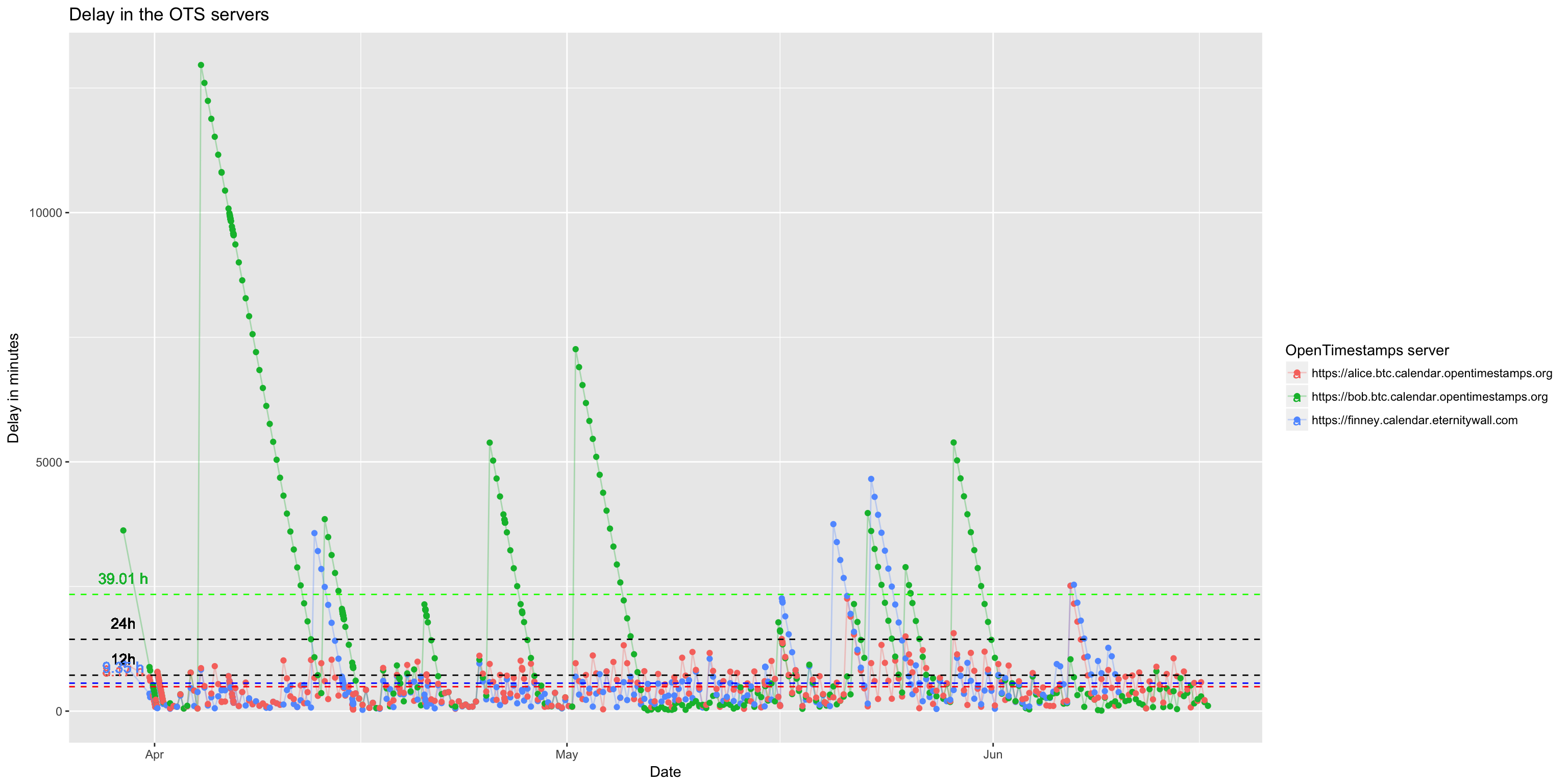
In this chart unfortunately we can see how some public server went down for maintenance/debugging activities generating long delays. Thanks to the architecture of OpenTimestamps this is not a big deal! Every timestamp request from the reference client is made to the 3 servers, what you really care of is the reply of the fastest one to write in the blockchain
For this reason we can plot just the minimum time for each timestamp, this is a good approximation of the time needed to publish a message. This is how OpenTimestamps protocol work, imagine to ask two servers (Alice and Bot) the same timestamp, the protocol return the timestamp of the minimal height block so, if Alice publish transaction before Bob, the protocol will return the timestamp on the block containing Alice’s transaction.
We can plot it using a dataset summarized by digest like in the following chunk.
my_dataLog_plot <- dataLog_plot %>%
   group_by(digest, blockchain) %>%
   summarize(timeCreated = min(timeCreated, na.rm = TRUE),
             siteUrl = siteUrl[which.min(timeCreated)],
             delta = delta[which.min(timeCreated)]
             )

ggplot(my_dataLog_plot[my_dataLog_plot$blockchain=="BTC", ], aes(x=timeCreated, y=delta)) +
   geom_line(alpha=0.3) +
   geom_point(aes(color=siteUrl)) +
   geom_hline(yintercept=720, linetype="dashed") +
   geom_text(aes(x=min(my_dataLog_plot[my_dataLog_plot$blockchain=="BTC", ]$timeCreated), y=720, label="12h", vjust=-1)) +
   geom_hline(yintercept=1440, linetype="dashed") +
   geom_text(aes(x=min(my_dataLog_plot[my_dataLog_plot$blockchain=="BTC", ]$timeCreated), y=1440, label="24h", vjust=-1)) +
   ggtitle("Minimum delay in the OTS servers") +
   xlab("Date") +
   ylab("Delay in minutes") +
   guides(color = guide_legend(title="OpenTimestamps server"))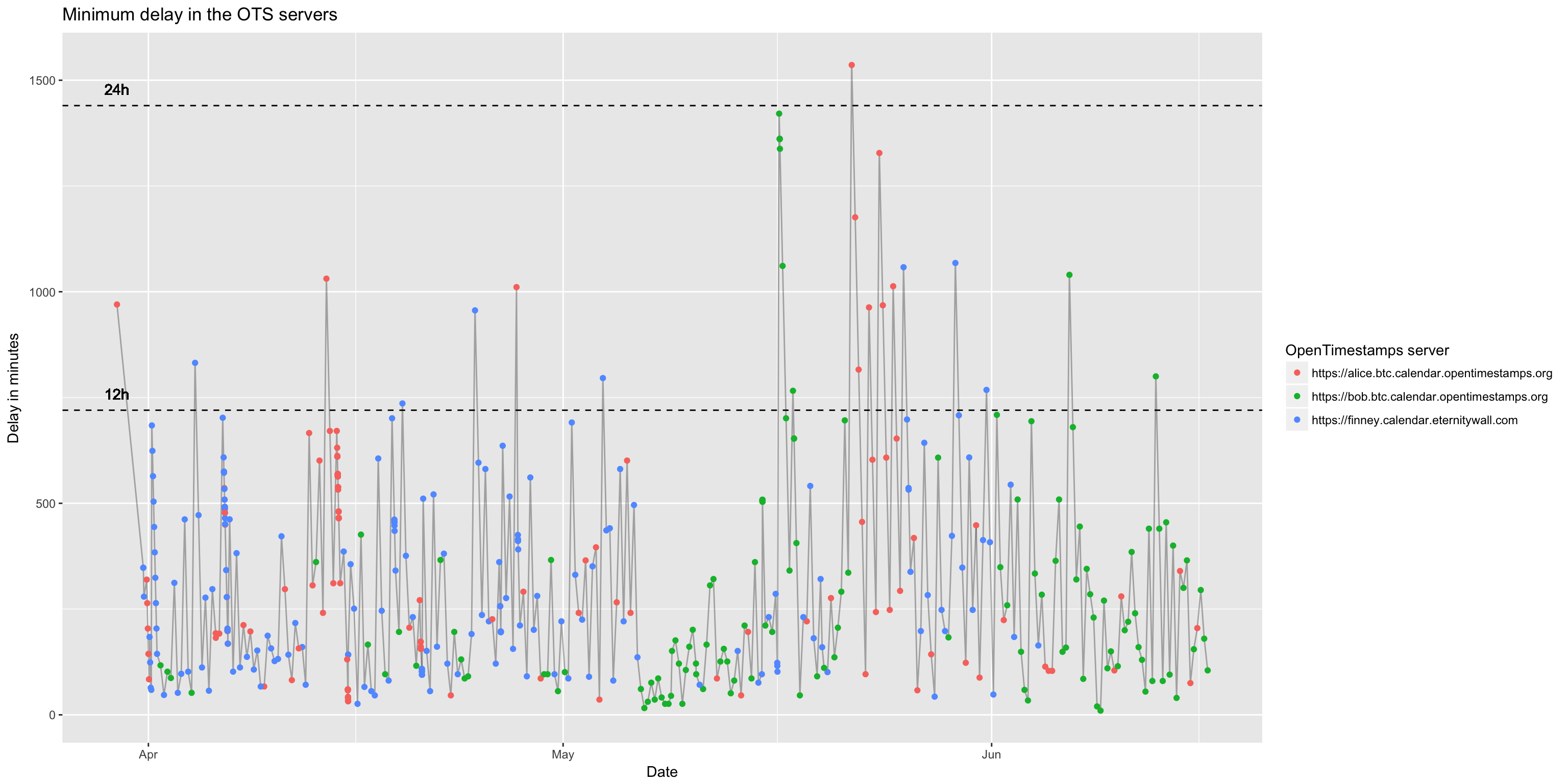
Remember that every server can decide:
- how many transaction do in a day,
- the amount of the fee for publish a message (adjustable using Replace By Fee approach better explained later).
In this chart we can also add the average confirmation time that represent the load of the blockchain.
load <- read.csv("https://api.blockchain.info/charts/avg-confirmation-time?daysAverageString=1&format=csv&scale=0×pan=30days", header = FALSE)
ggplot(my_dataLog_plot[my_dataLog_plot$blockchain=="BTC", ], aes(x=timeCreated, y=delta)) +
geom_line(data=load, aes(x=as.POSIXct(load$V1), y=as.numeric(load$V2)*5), alpha=0.8, linetype="dotted") +
geom_line(alpha=0.3) +
geom_point(aes(color=siteUrl)) +
geom_hline(yintercept=720, linetype="dashed") +
geom_text(aes(x=min(my_dataLog_plot[my_dataLog_plot$blockchain=="BTC", ]$timeCreated), y=720, label="12h", vjust=-1)) +
geom_hline(yintercept=1440, linetype="dashed") +
geom_text(aes(x=min(my_dataLog_plot[my_dataLog_plot$blockchain=="BTC", ]$timeCreated), y=1440, label="24h", vjust=-1)) +
ggtitle("Minimum delay in the OTS servers") +
xlab("Date") +
ylab("Delay in minutes") +
guides(color = guide_legend(title="OpenTimestamps server"))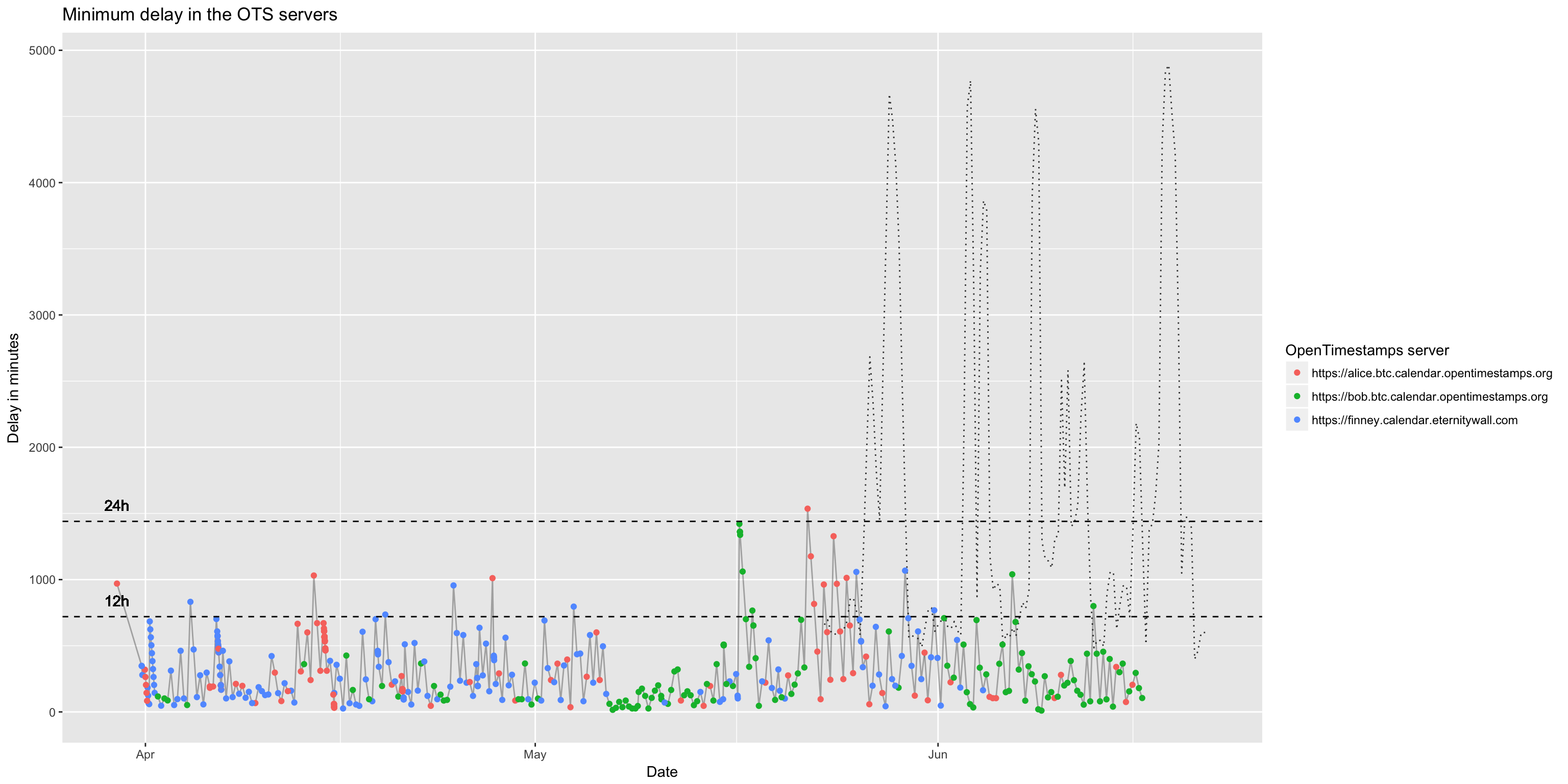
As we can see the average load has some effects on service speed but a good choice of fees can reduce the probability of an high delay.
Conclusions
We show how 3 OpenTimestamps free public servers perform in the real life and allow the publish of the transaction in less than 24 hours. With higher budget you can obviously obtain better performance, but even with infinite budget the maximum precision with bitcoin is +/- 2 hours.
If we represent the performance of the system using an histogram we can see how a large amount of timestamps are written in the chain in less than 12 hours and almost all timestamps are written and confirmed in the chain in less than 24 hours.
my_dataLog_plot$bar <- my_dataLog_plot$delta %/% 60
ggplot(my_dataLog_plot[my_dataLog_plot$blockchain=="BTC", ], aes(x=bar, fill=siteUrl)) +
   geom_histogram(bins = max(my_dataLog_plot$bar)+1) +
   ggtitle("") +
   xlab("Delay in hours") +
   ylab("Transactions") +
   guides(fill = guide_legend(title="OpenTimestamps server"))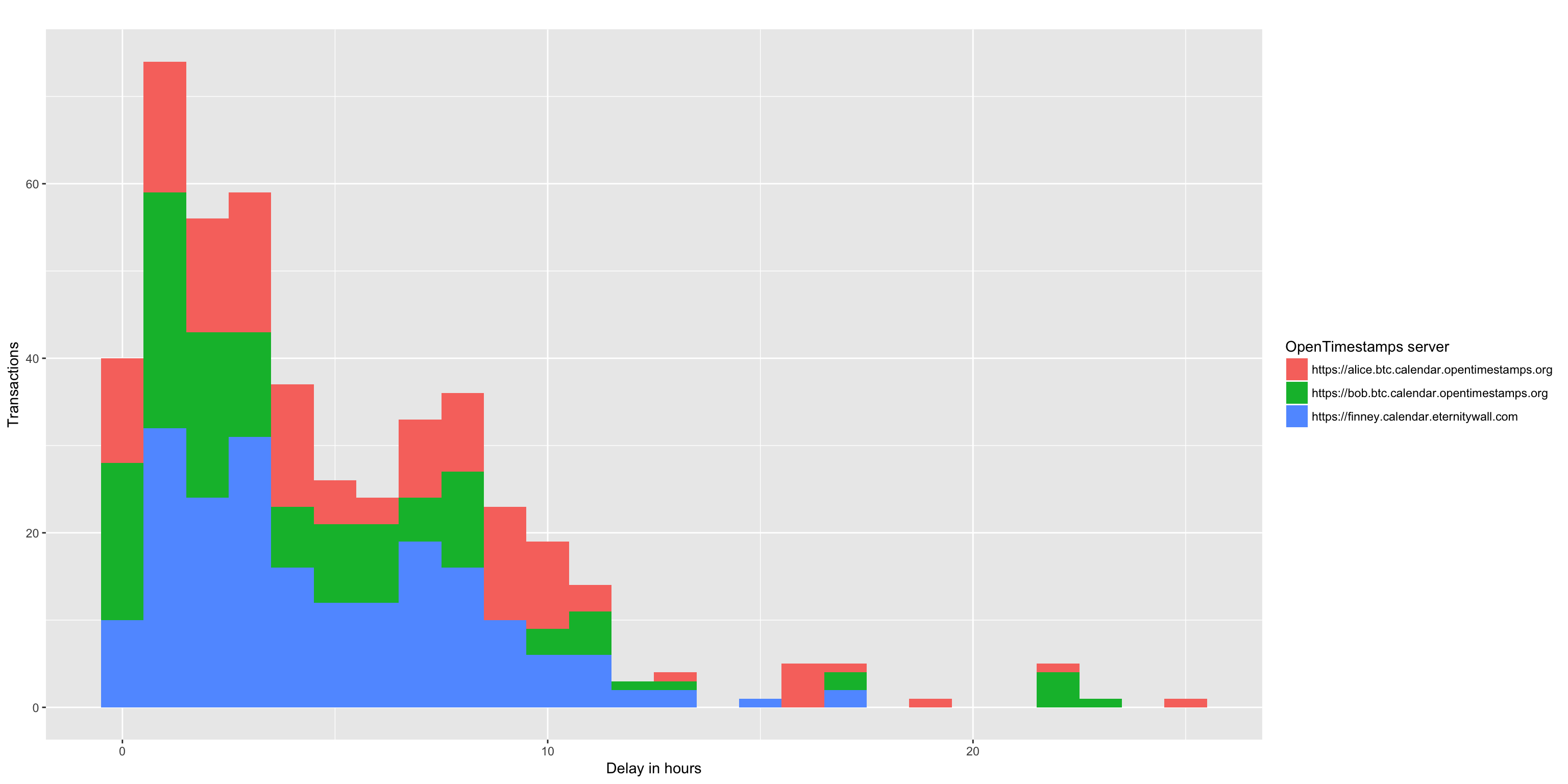
Or if you prefer in band of 6 hours…
my_dataLog_plot$bar_2 <- my_dataLog_plot$bar %/% 6
my_dataLog_plot$bar_2 <- factor(my_dataLog_plot$bar_2)
levels(my_dataLog_plot$bar_2) <- c("<6","6-12","12-18",">18",">18")
ggplot(my_dataLog_plot[my_dataLog_plot$blockchain=="BTC", ], aes(x=bar_2, fill=siteUrl)) +
   geom_histogram(bins = max(as.numeric(my_dataLog_plot$bar_2))+1, stat="count") +
   ggtitle("") +
   xlab("Delay in hours") +
   ylab("Transactions") +
   guides(fill = guide_legend(title="OpenTimestamps server"))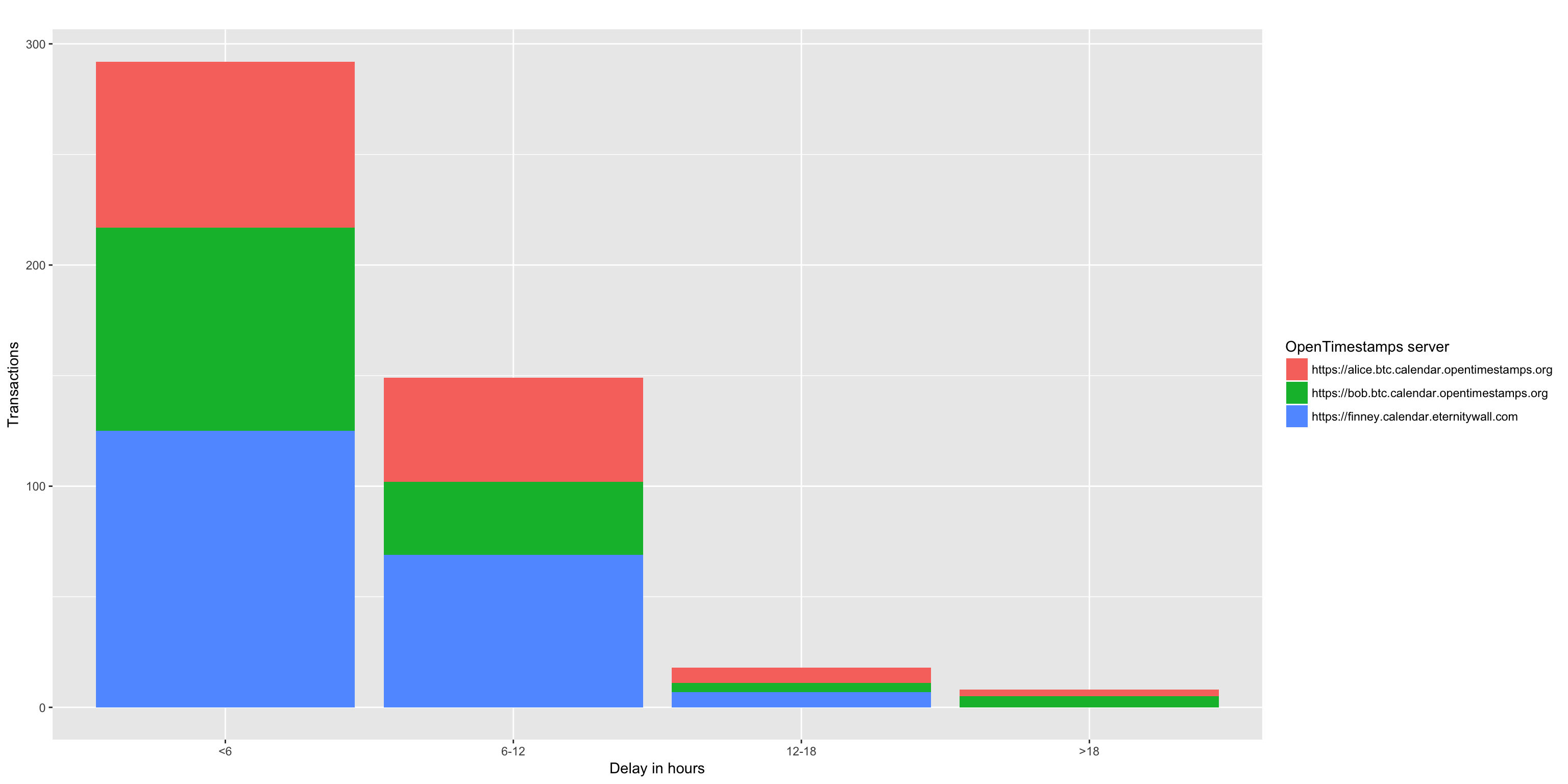
Not bad for public servers that work 24/365 with low fees, a lot of timestamp are processed in less than 12 hours and many in less than 6 (hey hey remember that a public server make a transaction every 6 hours …). Every transaction is processed in a day!
What makes possible this performances?
OpenTimestamps calendar may take long to create proofs but they will certainly do with a predetermined budget. The algorithm to create bitcoin transactions leverage the Replace By Fee feature.
By default, every node enforce the first seen rule on tx, but if RBF flag is set a transaction in mempool could be replaced by one spending the same input if it has higher fee.
When a calendar server needs to create a timestamping tx A, it starts with a minimum fee amount F. When the calendar receive a newly mined block, it checks if the tx A it’s in the block, if not, it creates another tx B using the same input as A but with a fee equal to transaction_fee_of_A + F. When another block is mined the algo repeats, until the transaction will be eventually confirmed.
With this algorithm, independently from the network condition, the Calendar server running budget is the number of blocks in a day (144) multiplied by F. What change depending on network conditions is the frequency of timestamping.
As we saw timestamping is possible using transaction on blockchain using the OpenTimestamps protocol, but remember:
- delay depends on the writing policy chosen (e.g. if you decide to write 4 times per day accept 12 hours granularity with acceptable fees) and
- delay depends on the fee chosen, if very low you accept to have a less precise timestamp.
A special thanks to Peter Todd and Riccardo Casatta for feedbacks and everyone who works on OpenTimestamps.